Exercise 3: exporting the attribute data and importing in Rstudio

So… we want to import the csv files we just made and downloaded in GEE to R, where we will do some basic data processing.

The camera_elevation.csv and camera_ndvi.csv should be in your google drive: these files you can download by navigating to google drive. Download both files and move them to a directory in which you want to do your work for this practical.

For example:

Great: so now we can shift to Rstudio

Open Rstudio. If all goes well, it should look something like this:

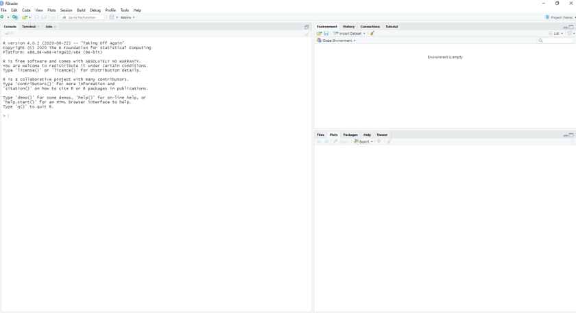
With on the left the console (where you execute single commands), on the top right a panel where you can see the variables in the ‘environment’. In the bottom right you can see the plots you make, but also e.g. the packages that are installed, or the help function.

We now have to do two things:

1. Import the two dataset
2. Build an R script to do some basic analysis

Importing the data and building a script

The first thing you need to do is build an empty R file where you will later put the commands you’ll use for analysis.

We can add simple code, as illustrated in the video below

Now let’s code ourselves: let’s first import the data.

# this is the file where we will list the commands needed for the analysis
# using a hashtag = comments 

#first let's see in which directory R is working now: 
getwd()

#this is probably not the directory you want (the directory where you stored your csv files). 
#so we need to change this. 
#in my case this is: 
setwd("C:/Users/lhjacob/OneDrive - UvA/UvA-Education/teaching/WFE/coursedocs2022/PRACT2") #note that R requires forward slashes in your path name

#check if it worked: 
getwd()


#let's now import the data, starting with the ndvi dataset: 
ndvi<-read.csv("camera_ndvi.csv")
#check out the dataset: which two columns are of interest to us? 
View(ndvi)

# now we can build simple code, to do some analysis
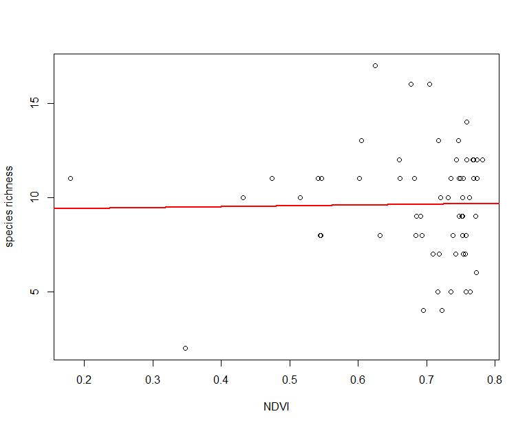
# first, let's plot
plot(x=ndvi$mean, y=ndvi$rich, xlab="NDVI", ylab = "species richness")

# then build a regression: 
regression_ndvi <- lm(ndvi$rich~ndvi$mean, data = ndvi)
summary(regression_ndvi)
# is the relationship significant? 

# plot regression line on scatterplot
abline(regression_ndvi, col="red", lwd=2)

After the execution, you should get something like this:

If this works, let’s do the final challenge of the day: repeat the above exercise, but now using the elevation data.

To start you on the right path, you can use the code below as a starting point. A ? means you’ll have to fill in the blank based on what you have learned above (so in analogy to the ndvi exercise) .

#let's now import the data, starting with the elevation dataset: 
elevation <-read.csv("?")
#check out the dataset: which two columns are of interest to us? 
View(?)

# now we can build simple code, to do some analysis
# first, let's plot
plot(x=?, y=?, xlab="?", ylab = "species richness")

# then build a regression: 
? <- lm(?~?, data = ?)
summary(?)
# is the relationship significant? 

# plot regression line on scatterplot
abline(?, col="red", lwd=2)