Exercise 3: exporting the attribute data and importing in Rstudio

So… we want to export the attribute data of our shapefile to a file that can be imported in Rstudio, e.g. a .csv file.

Luckily, that’s quite straightforward:

Great: so now we can shift to Rstudio

Open Rstudio. If all goes well, it should look something like this:

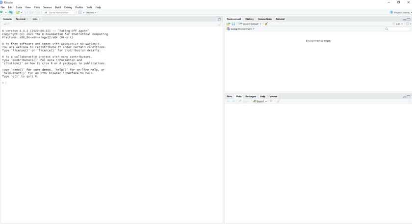
With on the left the console (where you execute single commands), on the top right a panel where you can see the variables in the ‘environment’. In the bottom right you can see the plots you make, but also e.g. the packages that are installed, or the help function.

We now have to do two things:

1. Import the dataset
2. Build an R script

Importing the .csv file we just made

Depending on the settings of your PC, you might need to adjust the decimal notation, or the seperator. If all is well, you now see the attribute information in the environment.

Building a script

Now we can start analyzing the data. The first thing you need to do is build an empty R file where you will later put the commands you’ll use for analysis.

We can add simple code, as illustrated in the video below

---

Note: In this exercise we are not considering the fact that the samples (watersheds) are spatially correlated: nearby watersheds will resemble each other more than watersheds that are further apart from each other. This is called “spatial autocorrelation”. Ignoring spatial autocorrelation (as we do here) could pose a problem in the sense that the observations (waterhsed) are not fully independent of one another, violating the assumption of our statistical test. Dealing with spatial autocorrleation is topic of courses at the master level. ***

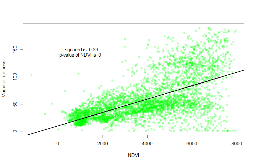
The plot is a bit ugly, so we can pimp it, and also plot the regression line. Copy paste the code below and execute it yourself:

# this is the file where we will list the commands needed for the analysis
# using a hashtag = comments 

# now we can build simple code, to do some analysis

#cleaning data
attributesNDVI_Richness<-na.omit(attributesNDVI_Richness)
attach(attributesNDVI_Richness)

# first, let's plot
library(scales) # if you get an error here, first install package 'scales' using install.packages('scales')
plot(NDVImean, richnessme, xlab = "NDVI", ylab = "Mammal richness", col=alpha("green",0.3), pch = 16)

# then build a regression: 
regression <- lm(richnessme~NDVImean, data = attributesNDVI_Richness)
summary(regression)


# plot regression line on scatterplot
abline(regression, col="black", lwd=2)

text(1000,150, paste("r squared is ", round(summary(regression)$r.squared,2)))
text(1000,140, paste("p-value of NDVI is ", summary(regression)$coefficients[8]))

After the execution, you should get something like this: