Welcome to the Second practical.
In this practical we will be using a combination of Google Earth Engine-QGIS-R to understand global biodiversity patterns. No need to worry, we’ll tackle it step by step. It is however essential that you found your way trough the first practical as we will start with getting (some of our) data there.
Step 1: Required softwares and datasets: overview
Softwares
As mentioned on the starting page, you’ll need QGIS, Rstudio and a working account for code editor.
Once you have installed QGIS, it will assume the language of your operating system. However, for troubleshooting, and communicating about issues as well as following tutorials, it is useful to have your interface in English. Changing the language can be done as follows:
Datasets
We’ll use following datasets:
| Dataset | Type | Source | Access point |
|---|---|---|---|
| Mammal species richness - Global | Raster | Jenkins et al. 2015 | biodiversity.org |
| NDVI map - Global | Raster | Modis Imagery | Google Earth Engine: see below |
| Watershed delineations - Global | Vector | WWF | Google Earth Engine: see below |
Step 2: accessing the data
MAMMAL SPECIES RICHNESS
The easiest dataset to access is the raster file for Mammal Species Richness: just clicking on the link in the table should result in an immediate download of a ZIP file. Unpacking this gives you access to a raster file: we’ll only need the tiff file with following name: Richness_10km_MAMMALS_mar2018_EckertIV.tif
For the two other maps we can use Google Earth Engine to access them.
NDVI MAP
We’ll start with visualizing and downloading the NDVI map: Google Earth Engine allow to upload any Image you make to your google drive: once on your drive, you can download it from there.
The whole google earth engine code is here below, with each of the lines commented: make sure you understand what all the different parts are for, what they do, and try to execute the code yourself using your own google earth engine account:
/// we define the area for which we want to download data:
var clip =  ee.Geometry.BBox(-180, -60, 180, 60); // we use the function ee.Geometry.BBox to define a bounding box


/// we define the dataset (ImageCollection) we are interested in, and already filter a few years from it:
var dataset = ee.ImageCollection('MODIS/006/MOD13A2')
                  .filter(ee.Filter.date('2015-01-01', '2018-12-31'));

/// the MODIS image collection we just defined contained much more than only NDVI. We can check what is in this dataset by using *print*:
print(dataset);
// the info on what is in the datset now appears in the console, where you can click on the item and explore


/// so let's just select NDVI
var ndvi = dataset.select('NDVI');
print(ndvi);
// you can see in the console, that it is still an image collection, because it contains one NDVI image per 16 days!

// so we'll have to take the average over the whole set:
var mean = ndvi.reduce(ee.Reducer.mean());
print(mean);
// indeed: taking the average *reduces* the image collection to an Image: this we can export to our drive
// but... let's first visualize:-)


// define the minimum, maximum and the colour pallette:
var ndviVis = {
  min: -1000,
  max: 9000.0,
  palette: [
    'FFFFFF', 'CE7E45', 'DF923D', 'F1B555', 'FCD163', '99B718', '74A901',
    '66A000', '529400', '3E8601', '207401', '056201', '004C00', '023B01',
    '012E01', '011D01', '011301'
  ],
};

//center the map, and add the ndvi map:
Map.setCenter(6.746, 46.529, 2);
Map.addLayer(ndvi, ndviVis, 'NDVI');


// Export our 'mean' to your google drive: we have to define the region (clip), the scale: here we take 5km at the equator, and give it a name
Export.image.toDrive({
  image: mean,
  description: 'meanNDVI_MODIS',
  scale: 5000,
  region: clip,
  fileFormat: 'GeoTIFF'
});
// after running this it should appear in your 'tasks' here to the right: click on 'run'
After running this code, a new task should appear on the right panel: executing this will allow a geo-tiff file (type of raster file) to load in your google drive: from here you can download it to your PC:-).
Note that the values range from -2000 to 8000: this is different from what you know from the classes in remote sensing (NDVI typically ranging between -1 and 1): this is because, for data storage and processing reasons, it is more interesting to store all values as integers and assign a scaling factor (in this case a value of 1000). All the integers you see on the map thus in reality represent the NDVI*1000
WATERSHED VECTOR FILE
For the exercise on Biodiversity patterns, we’ll use watersheds as spatial units. Watersheds can be constructed at various scales (e.g. you could consider the whole catchment of the Amazone river, or you could consider the smaller catchments of its tributories). Watersheds can be a convenient spatial scale because they represent a bio-physical unity (e.g. in contrast to the boundaries of a province or country, representing administrative units). The fact that you can decide at which scale you define your watersheds also makes it (at least scale-wise) a rather flexible unit.
To download the shapefile of the hydrosheds by WWF, we’ll follow a very similar protocol as the NDVI map above, but tailored to vector data (features in GEE).
/// define the region of interest (ROI):
var clip =  ee.Geometry.BBox(-180, -60, 180, 60);


/// define the dataset of interest: in our case the watersheds by WWF, at the 5th level of detail (highest level = 12)
// we also clip the features to the ROI
var watersheds5 = ee.FeatureCollection("WWF/HydroSHEDS/v1/Basins/hybas_5").filterBounds(clip);

//OK, let's visualize:
Map.addLayer(watersheds5);


// Export the FeatureCollection to a shape-file.
Export.table.toDrive({
  collection: watersheds5,
  description:'hydrosheds5',
  fileFormat: 'SHP'
});
PUTTING EVERYTHING TOGETHER
The MODIS raster NDVI file and the shapefile for the hydrosheds (download all files named ‘hydrosheds5’, not only the .shp file) can now be downloaded from your google drive.
Unzip where needed, and put all information in one folder, similar to the example below:
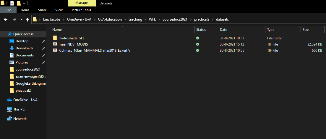
Now we are ready for the next step: loading all the data in to QGIS and starting the analysis