View on GitHub

World-Food-and-Ecosystems

Step 2: Data Retrieval

The easiest set to download are the administrative boundaries of Belgium, this is through a direct download here

Unzip the file: you’ll see it countains shapefiles on many administrative levels: only those at the 0th level are of interest to us:

make sure all files coded with BEL_adm0 (so all files starting with these letters, regardless of the file extension) are stored in an appropriate folder (e.g. a folder ‘Belgium’ in the folder you made for this practical.

Now that we have the shapefile, let’s open in it in QGIS and subdivide it in smaller spatial units (polygons in the shape of gridcells) that we can use to do our analysis.

Because the shapefile of Belgium is referenced in WGS84 ( so it has geographical coordinates in degrees rather than x,y coordinates in meters) the unit of subdivision is also in degrees. Note that it would be more correct to convert all layers to a projected coordinate system (e.g. UTM). For the purpose of this exercise, we’ll keep all data in WGS84. To subdivide the territory, we’ll need two functions: Create Grid function you’ll find under the ‘vector’ tab, and finally, you’ll need to remove all the cells that (partially) fall outside of the boundaries of this country. The videos below show you how’

Now, let’s try a ‘point and click’ plugin that enables an OSM API plugin in QGIS.

We’ll first need to install this plugin “QuickOSM”: this is shown in the video below.

Great, now we can actually use the plugin to download the rivers of Belgium. Following steps/details are needed:

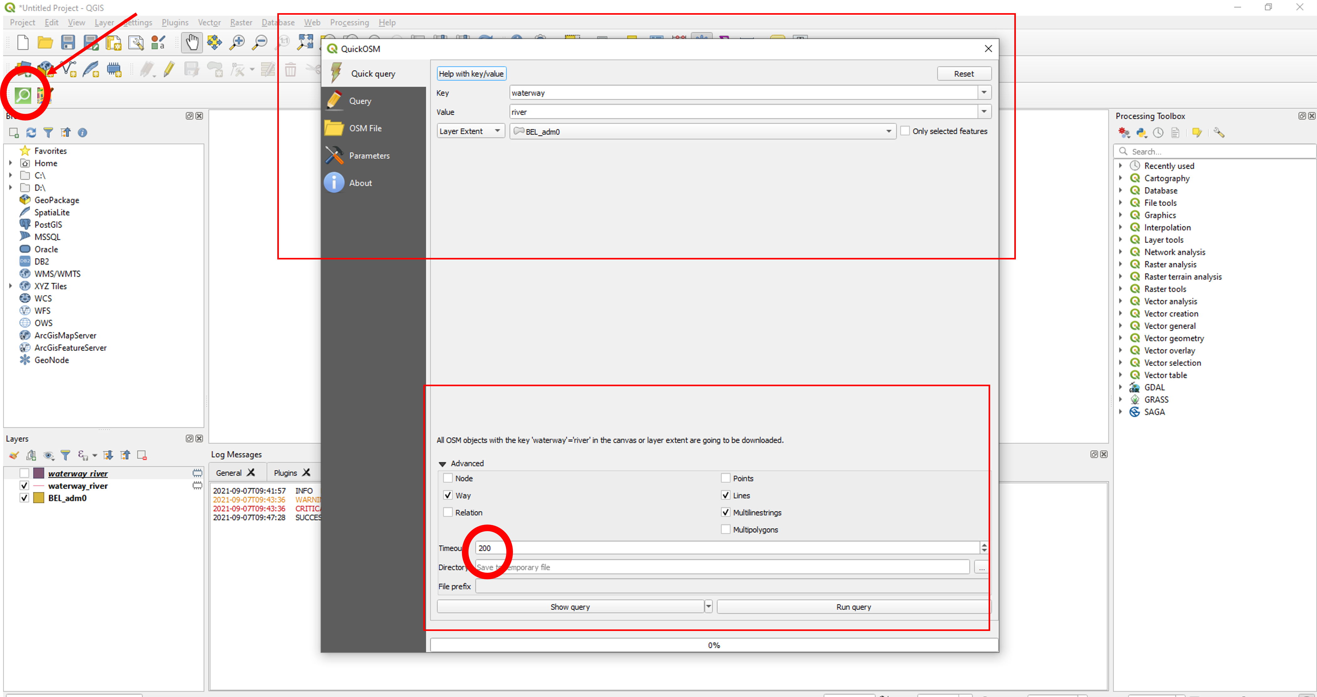
Open the plugin (the green magnifying glass in the upper left corner) Rivers in OSM belong to the Key ‘Waterway’ and the Value ‘River’. For the location, we want to use the administrative boundary of belgium we just downloaded Because the data we try to access is quite a large set, we’ll increase the time allowed (before an error is trown) to 200 seconds (under advanced settings). We also untick the ‘node’box, the ‘relation’ box, the ‘points’ box and the ‘mulitpolygons’ : rivers are coded as ‘Ways’in OSM and as lines or multilinestrings, so by unticking the other boxes, we’ll remove unnecessary searches. The Final interface of the plugin should look like the figure below now you can click on Run query and wait: if all goes well, the layer should load in QGIS if you execute too many queries/downloads in a short amount of time, the server might refuse to execute. In case of persistant difficulties, you can also download the dataset here.

osmplugin

Now that we have our river layer, we can download the raster fill for topographic diversity. Luckily, we already know how, as this layer is available in GEE, so we can clip the image we need, and export it to our google drive, and from there, download it: ! Note that this could take a few minutes: in the meantime you could further explore the papers that are on canvas.

var belgium_window = 
    ee.Geometry.Polygon(
        [[[2.51, 51.6],
          [2.51, 49.49],
          [6.48, 49.49],
          [6.48, 51.6]]]);

var dataset = ee.Image('CSP/ERGo/1_0/Global/ALOS_mTPI'); //load the mTPI image
var alosMtpi = dataset.select('AVE'); //select the correct band (there is only one)
var topo = alosMtpi.clip(belgium_window); //clip with a box containing belgium
print(topo);

Map.addLayer(topo);

//what is the resolution? 
print(topo.projection().nominalScale());

Export.image.toDrive({
  image: topo,
  description: 'topodivALOS',
  scale: 270,
  fileFormat: 'GeoTIFF'
});

Now comes the most tricky data to download: we’ll access the GBIF API through the command line in R.

Open Rstudio and make a new .R file in which you will copy and (slightly) adjust the code to access the gbif data. Note, if you get warnings or error messages regarding packages that are needed but not installed, please install them using the install.packages function we also use below.

Step 1, we will simply install and load the packages we need:

install.packages('rgbif') 
install.packages('sp') 
install.packages('rgdal') 
library(rgbif)
library(sp)
library(rgdal)

Step2: we simply set the directory in which R should read and write data: adjust what is between “” to your own path

setwd("C:/Users/LHJACOB/OneDrive - UvA/UvA-Education/teaching/WFE/coursedocs2021/practical3/") #note that R only accepts forward slashes in path. 

Step3: now we are ready to access the gbif data.

We want Raccoon (Procyon Lotor) in Belgium, and only sightings with coordinates. If you searh Procyon Lotor in gbif.org you will get to following page: https://www.gbif.org/species/5218786 the last few numbers in this url is the taxonKey of the raccoon: a key that gbif uses to identify taxons Now we have all info to build a query for the raccoon in Belgium, with coordinates:

#BUILD THE QUERY; 
result <- occ_download(pred('taxonKey', 5218786), pred('hasCoordinate', TRUE), pred("country", 'BE'), email = "FILL IN YOUR EMAIL HERE", pwd="FILL IN YOUR PASSWORD HERE", user="FILL IN YOUR USERNAME HERE")

#DOWNLOAD THE METADATA
occ_download_meta(result)   # this step takes some time: repeat once every minute or so to check updates

Once this last command changes from status ‘preparing’ or ‘running’ to ‘succeeded’ you can move to the download

data <- occ_download_get(result, overwrite = T) #download the data
raccoons<-occ_download_import(data) #import the data

This data has A LOT of columns, many of which we don’t need, so let’s simplify, and then only select those sightings that occur since 2015

raccoons<-as.data.frame(cbind(raccoons$decimalLatitude,raccoons$decimalLongitude,raccoons$year))
colnames(raccoons)<-c("lat", "lon", "year")
raccoons<-raccoons[which(raccoons$year>2014),]

Great, only one thing left to do: export the data as a shapefile: This is relatively simple: we’ll have to explicitly tell R where to find the coordinates, and then write the file:

coordinates(raccoons)<-cbind(raccoons$lon,raccoons$lat)
writeOGR(obj=raccoons, dsn=getwd(), layer="raccoons", driver="ESRI Shapefile") # this is in geographical projection

Now, if all is well you should have the point shapefile of the raccoons, the line shapefile of the rivers, the polygon shapefile of the boundaries of belgium and the tiff raster file with the topographic diversity: check if you have all the data in one place (e.g. the folder you made specifically for this practical exercise) using the table:

Dataset	Type	Source	Access point
Raccoon sightings	Vector:points	GBIF	GBIF API in R
River Network	Vector:lines	Open Street Map	OSM API in QGIS
Topographic Diversity	Raster	derived from the ALOS DEM	Google Earth Engine
Boundary of Belgium	Vectory: polygon	OSM	Direct download: https://biogeo.ucdavis.edu/data/diva/adm/BEL_adm.zip

**Great, we can move to the geo-processing in QGIS